Abstract
- A daily long/short strategy based on Augmento sentiments and backtested on Bitmex XBTUSD generated a positive return between 2017 and 2019
- The signal which generated positive returns in a stable manner over the test period is based on a ratio of bullish and bearish Bitcoin sentiment, while signals based on random combinations of sentiments do either not generate positive returns or exhibit random performance
- Main caveat is that trading fees were not included for this research note
Creating algorithms to trade Bitcoin is hard, and finding good data that is independent of the price but still correlated with the market is even harder. Sentiment data could be the answer, but it’s often hard to use for algorithmic trading, and rarely provides more than an unsophisticated positive or negative signal.
Augmento sentiment data offers a broad multi-dimensional view on the cryptocurrency market, packaged in the same candle format as market data from the top cryptocurrency exchanges. In this article, we’ll load some data, develop a simple trading signal based on these data, backtest the signal using a basic market model, and evaluate the results.
All code can be found on Github.
Loading the data
The Bitmex API provides a super simple way to get historic candlestick data (amongst other things) using the /trade/bucketed endpoint. Here’s an example for getting 1-hour candlestick data between 2019–01–01 00:00and 2019–01–02 00:00:
params = {
"symbol" : "XBt",
"binSize" : "1h",
"count" : 10,
"start" : 0,
"startTime" : "2019–01–01T00:00:00Z",
"endTime" : "2019–02–01T00:00:00Z",
}
url = "https://www.bitmex.com/api/v1/trade/bucketed"
r = requests.get(url, params=params).json()</code></pre>Looking at the response:
[{'close': 3693,
'foreignNotional': 24965778,
'high': 3695.5,
'homeNotional': 6766.36017934,
'lastSize': 20,
'low': 3682.5,
'open': 3686.5,
'symbol': 'XBTUSD',
'timestamp': '2019–01–01T00:00:00.000Z',
'trades': 10718,
'turnover': 676636017934,
'volume': 24965778,
'vwap': 3689.7646},
...
{'close': 3712.5,
'foreignNotional': 37688803,
'high': 3722,
'homeNotional': 10149.23641118001,
'lastSize': 167,
'low': 3702.5,
'open': 3703,
'symbol': 'XBTUSD',
'timestamp': '2019–01–01T09:00:00.000Z',
'trades': 14849,
'turnover': 1014923641118,
'volume': 37688803,
'vwap': 3713.4688}]</code></pre>We’ve included a script for loading example XBTUSD data and running examples and tests. Just go to the root folder and run:
python3 examples/2_load_bitmex_example_data.py</code></pre>Getting data from the Augmento API is just as easy. For Twitter activity about Bitcoin for the same period:
params = {
"source" : "twitter",
"coin" : "bitcoin",
"bin_size" : "1H",
"count_ptr" : 2,
"start_ptr" : 0,
"start_datetime" : "2019–01–01T00:00:00Z",
"end_datetime" : "2019–02–01T00:00:00Z",
}
endpoint_url = "http://api-dev.augmento.ai/v0.1/events/aggregated"
r = requests.get(endpoint_url, params=params).json()</code></pre>Again looking at the data:
[{'counts': [1, 1, 0 ... 0, 2, 17],
'datetime': '2019–01–01T00:00:00Z',
't_epoch': 1546300800},
...
{'counts': [0, 1, 0, 0 ... 0, 7, 19],
'datetime': '2019–01–01T01:00:00Z',
't_epoch': 1546304400}]</code></pre>Each element in the counts list gives the number of Tweets classified with a given topic or sentiment in the bin starting with the given timestamp. To get a list of these topics and sentiments, query the topics endpoint:
r = requests.get("http://api-dev.augmento.ai/v0.1/topics").json()
Response is a dictionary of the topics and sentiments, with the key giving the index of the topic or sentiment in the counts list above:
{'0': 'Hacks',
'1': 'Pessimistic/Doubtful',
'10': 'Institutional_money',
'11': 'FOMO',
...
'90': 'Airdrop',
'91': 'Optimistic',
'92': 'Negative'}
Again, we’ve included scripts in our Github repo for loading this data, just run the following to save some data locally:
python3 examples/0_load_augmento_example_data.py
python3 examples/1_load_augmento_example_info.py
Viewing the data
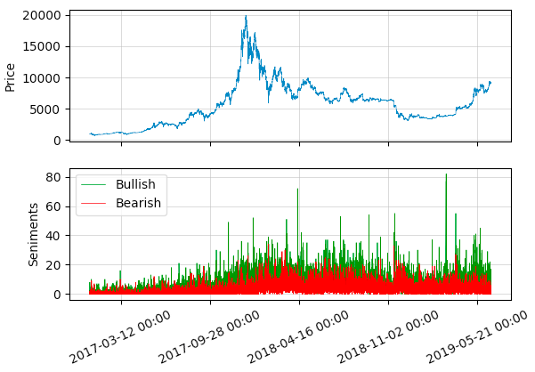
Once we’ve loaded some example data, we can plot some of the signals — in this case, we picked the Bullish and Bearish sentiment signals — against the price:
python3 examples/3_plot_augmento_example_data.pyThis gives us a graph of the price of Bitcoin (actually XBTUSD on Bitmex) against the Bullish and Bearish counts:
Interestingly, the volume of Bullish and Bearish Tweets increases during the boom towards the end of 2017, and falls off again (though only slightly) around the beginning of 2019 after the big price drop. This is consistent with the idea that social media activity may have been high during the hype.
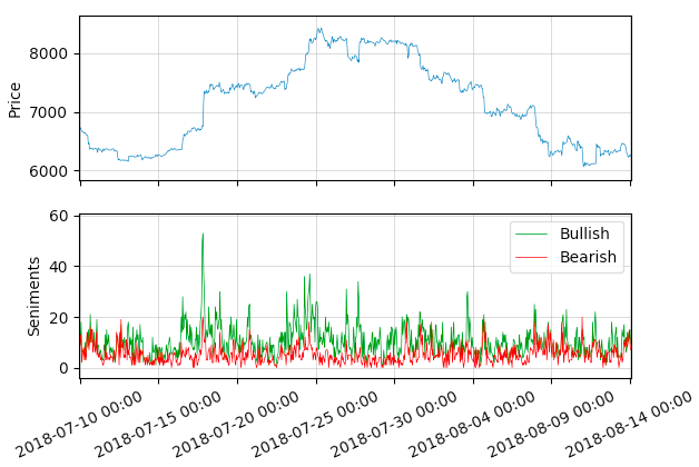
Let’s look a bit more closely at a random stretch of the data:
Notice the higher count of Bullish Tweets during the rise, and the reduced Bullish Tweets during the fall.
Creating a strategy
Though there are some clear trends in the sentiment data that correspond with the price movement, there don’t appear to be any clear buy or sell indicators. We’re going to have to do some processing to get a signal.
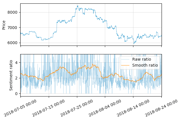
We can start by picking the signals we want to use, in this case, the Bullishand Bearish Bitcoin sentiments. Our hypothesis is that when the ratio of Bullish sentiment to Bearish sentiment is high the price is likely to rise, with the price falling when the opposite is true. Looking at the ratio of Bullishsentiment to Bearish sentiment, the ratio is very spiky with a clear bias; still far from the smooth stationary signal we’re looking for.
We can smooth the signal by taking a Simple Moving Average (SMA) for the past 7 days. The choice of a 7 day SMA was arbitrary, but note how this is still correlated to some extent with the price:
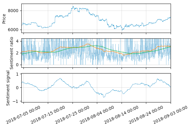
This smooth signal looks much better, but still doesn’t provide a clear buy or sell indicator. An example indicator could be an oscillating signal with a mean of ≈0.0, indicating a long position when >0.0, and a short position when <0.0. One way to generate this signal would be to calculate a rolling mean of the smooth signal x, and compare the last value xʷ in that window to the mean:
Here we are also dividing the signal by the standard deviation of the smooth signal x, so we get an output y which falls roughly within bounds [-2.5, 2.5].
This gives us a nice stationary sentiment signal that looks like it may correlate with price movements, and which could be used as the basis of a strategy. Considering that the price and sentiment signals are independent; it’s fairly surprising how correlated they are.
Backtesting the strategy
Having developed a signal, we can now create a strategy based on that signal, and test it in a simple market simulation.
To run our backtest, we look at the price and PnL (basically the total wallet value) at every step, and — depending on whether our signal indicates to go long or short in the previous step — calculate the new PnL depending on the change in the price from the previous step. We also subtract a small percentage of the total PnL each time there is a trade to simulate the trade fee. Pseudocode below:
for i in steps:
 if s[i-1] > 0.0:
  pnl[i] = (p[i] / p[i-1]) * pnl[i-1]
 else if s[i-1] < 0.0:
  pnl[i] = (p[i-1] / p[i]) * pnl[i-1]
 else if s[i-1] = 0.0:
  pnl[i] = pnl[i-1]

 if sign(s[i-1]) != sign(s[i-2]):
  pnl[i] = pnl[i] - (pnl[i] * trade_fee)
Note that the calculation of the PnL is only approximate, and varies depending on the exchange and the asset. Note also that we are careful to make sure the backtest is causal, using the sentiment score value in the previous step to set the position for the current step for which the new PnL is calculated.
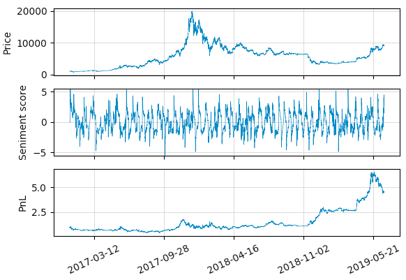
Once we’ve set up our backtest, we can run it over some historical price and sentiment data for a pair of sentiments/topics and a given set of parameters. The plot below shows the performance of a Bullish/Bearish strategy, with a window size of 168 hours (7 days) for both the first and second rolling windows (SMAs). Note that the sentiment score has also been scaled by the standard deviation of the second rolling window for each window, so it stays roughly within the bounds -5.0 to 5.0.
The backtest above is also included in the repo:
Note again that the PnL calculation is only approximate, and we didn’t account for fees or slippage so it is unlikely to be true to life, but it’s a good start considering the window parameters were picked at random.
It would also be wise to run a backtest on a topic/sentiment pair picked at random to provide a basic control for our experiment above. Here, we’ve backtested the same strategy on the Rumor/Technical_analysis pair:
The final PnL here is much lower, and the Sharpe ratio is much worse on inspection (the PnL is generally flat, with occasional large jumps). This provides some evidence that the relatively good performance of our Bullish/Bearish experiment was consequent on our choice of topic/sentiment pair, rather than because of some discrepancy in our model.
Caveats and further research
We showed how we can use noisy raw non-stationary data to develop a signal suitable for a trading strategy, and how we can use a backtest to estimate the strategy performance. It should be noted again that we are ignoring several important elements here, such as trade fees, slippage, and market liquidity; this will be covered in future researcj.
In the next research note, we are going to review the signal and backtest we have created, and see if we can optimise it by selecting other topic/sentiment pairs, and testing various window size parameters. We will also be stress-testing these parameters by looking at how they perform in a range of market conditions, and after adding random noise.
All the code for the experiments above can be found on Github, together with documentation for the Augmento API. Historical sentiment data is also freely available for Bitcoin on the API from 2014 up until the last 30 days, as well as historical data with various starting dates for all the other major coins (Ethereum, Ripple, Dash, Stellar, 0x, etc.).


